Here’s the easiest way to hide and show cells using checkboxes in Google Sheets.
First, we have to remember when you check a checkbox the value is –
TRUEAnd when you uncheck the box the value is –
FALSE
Here’s the spreadsheet we’ll be using. Feel free to make a copy of this spreadsheet to follow along.
Hide and Show Cells Using Checkboxes | Formula Method
Here we’ll use this formula in a cell
IF(B2, “MESSAGE WHEN TRUE”,”MESSAGE WHEN FALSE”)
Remember,
IF(B2) is equivalent to
IF(B2=TRUE)but isn’t equivalent to
B2 = “TRUE”
TRUE is from a boolean (true/false) value, and “TRUE” is a literal string. We want this formula to hide data when the checkbox is FALSE, so let’s adjust the formula and remove “MESSAGE WHEN FALSE” and instead just have two quotations.
IF(B2, “Customer Notes”,””)
Lastly, B2 is the cell where the checkbox is.
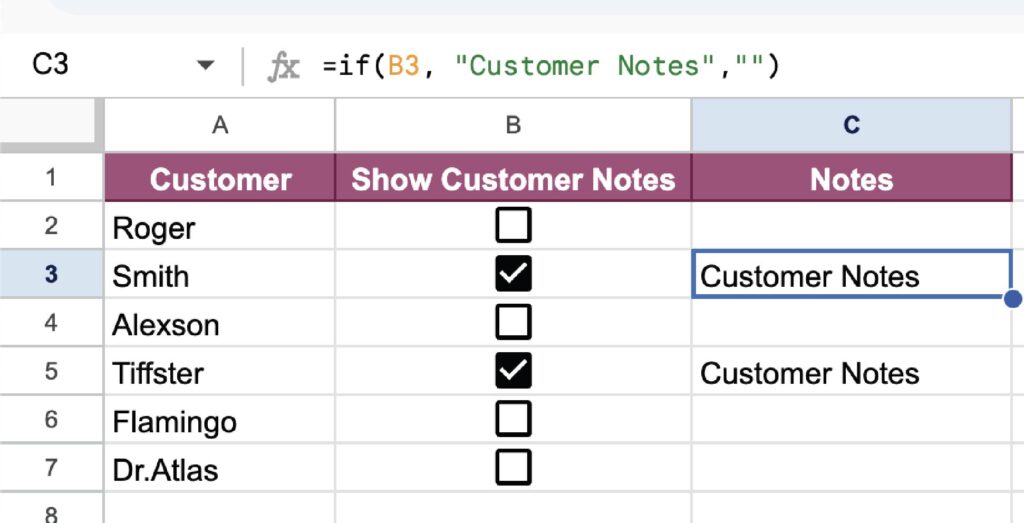
This method is easy, but in some cases not the most ideal. Since it’s a formula, you can’t freely type your notes as you need. The next example is a more robust way.
Hide and Show Cells Using Checkboxes | Conditional Formatting
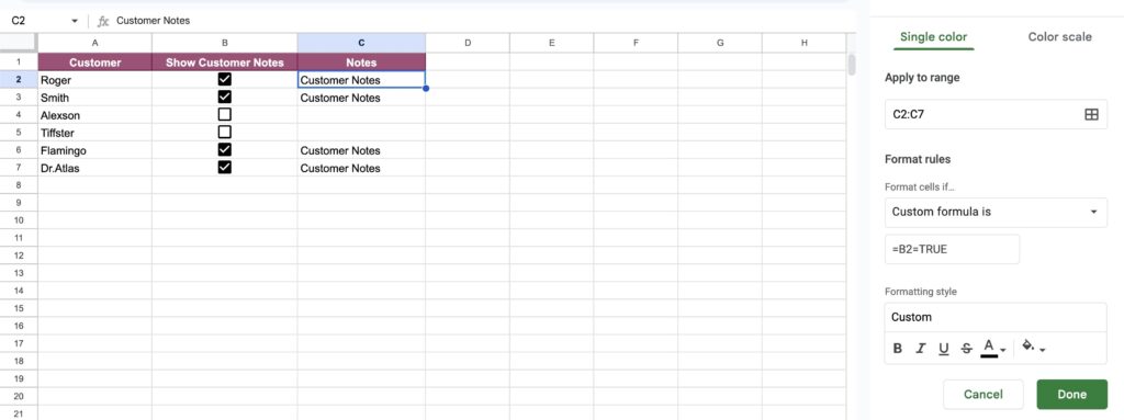
Using conditional formatting to hide and show cells with checkboxes allows us to have free range over editing any cell we desire, without worrying about overwriting a formula. This method is very similar to what we did above, but instead, we’re placing the formula inside this conditional formatting tool and matching the text to the background to make it appear invisible.
Here’s the steps
- Format -> Conditional Formatting
- Format rules -> Custom formula is
- =B2=TRUE (replace B2 with the checkbox cell)
- Formatting style – > match the text color to the background color
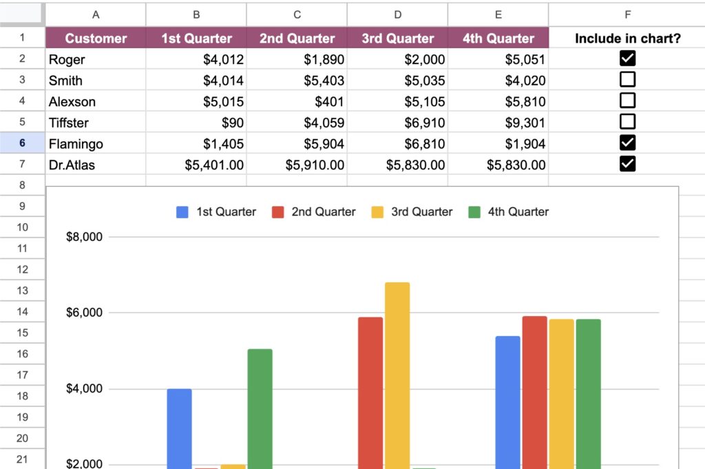
This is just scratching the surface of the opportunities checkboxes present for Google Sheets. We can also use checkboxes to show and hide data from a chart.
We can also use checkboxes to highlight certain checked checkboxes (with conditional formatting).

Enjoy these easy methods to hide and show data using checkboxes!
