Checkboxes are a powerful tool that functions way beyond just visualizations. Adding checkboxes in Google Sheets is a great way to improve organization, manage your spreadsheets, simplify data, and more! We’ll cover the simple process of adding these checkboxes in Google Sheets as well as exploring useful functionalities.
Insert checkboxes | How to add checkboxes in Google Sheets
- Select cell(s) you want to add checkboxes to
- Insert (menu bar) > Checkbox
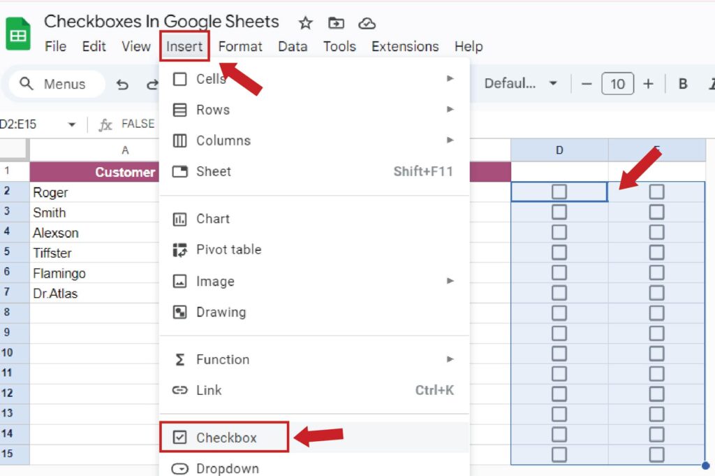
Just like that, you have added your checkboxes! Cool, right? Google Sheets has some additional documentation, like adding custom values to these checkboxes. Now that your question ‘How to add checkboxes in Google Sheets’ is answered, it’s time to dive deeper.
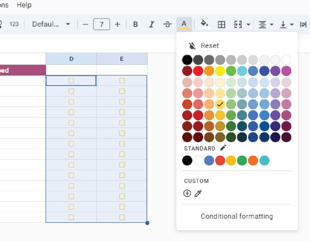
Customize checkboxes
Checkboxes in Google Sheets has some limits with customization, however, treat it like normal text. For example, adjust the size (same as font size tool), the color (same as text color tool), alignment is the same, and much more.
Examples with checkboxes
Here’s the fun part – you have unlimited options! A checkbox may not look like it has values, but it does. If it’s checked, it’s value is TRUE, and FALSE if unchecked. You can customize this if needed. Also, it’s fine if you just use checkboxes for the visual appeal. I have step-by-step videos of these checkbox examples. Watch them here.
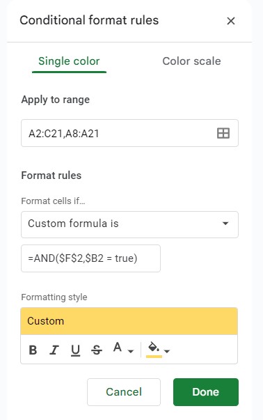
Highlighter with Checkboxes
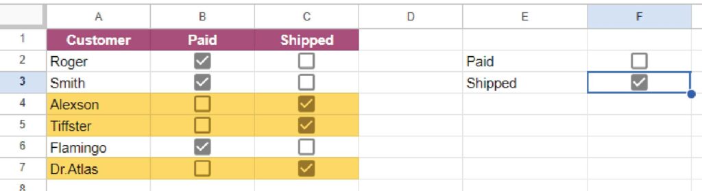
As you see, I have two additional checkboxes to the right to toggle between highlighting ‘Shipped’ and ‘Paid. You need two conditional format rules for each cell you want to be highlighted.
=AND($F$3,$C2 = true)
Highlights the ‘Shipped’ Column, and checks first to see if F2 is highlighted.
=AND($F$2,$B2 = true)
Same thing but for the ‘Paid’ column. Here’s what one rule should look like –
Hide / Show Cells with Checkboxes
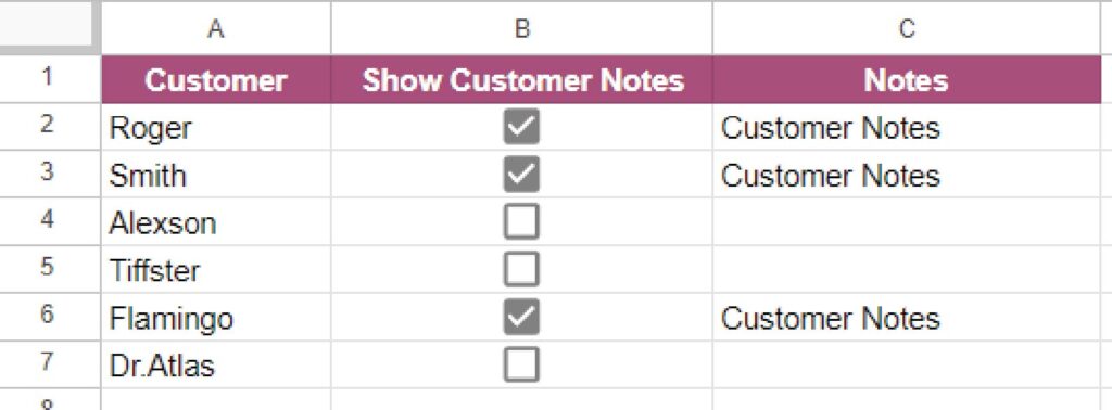
Very simple, starting in C2 I have the formula
=if(B2, “Customer Notes”,””)
Saying if B2 is the same thing as saying if B2 is true.
Dynamic Charts with Checkboxes
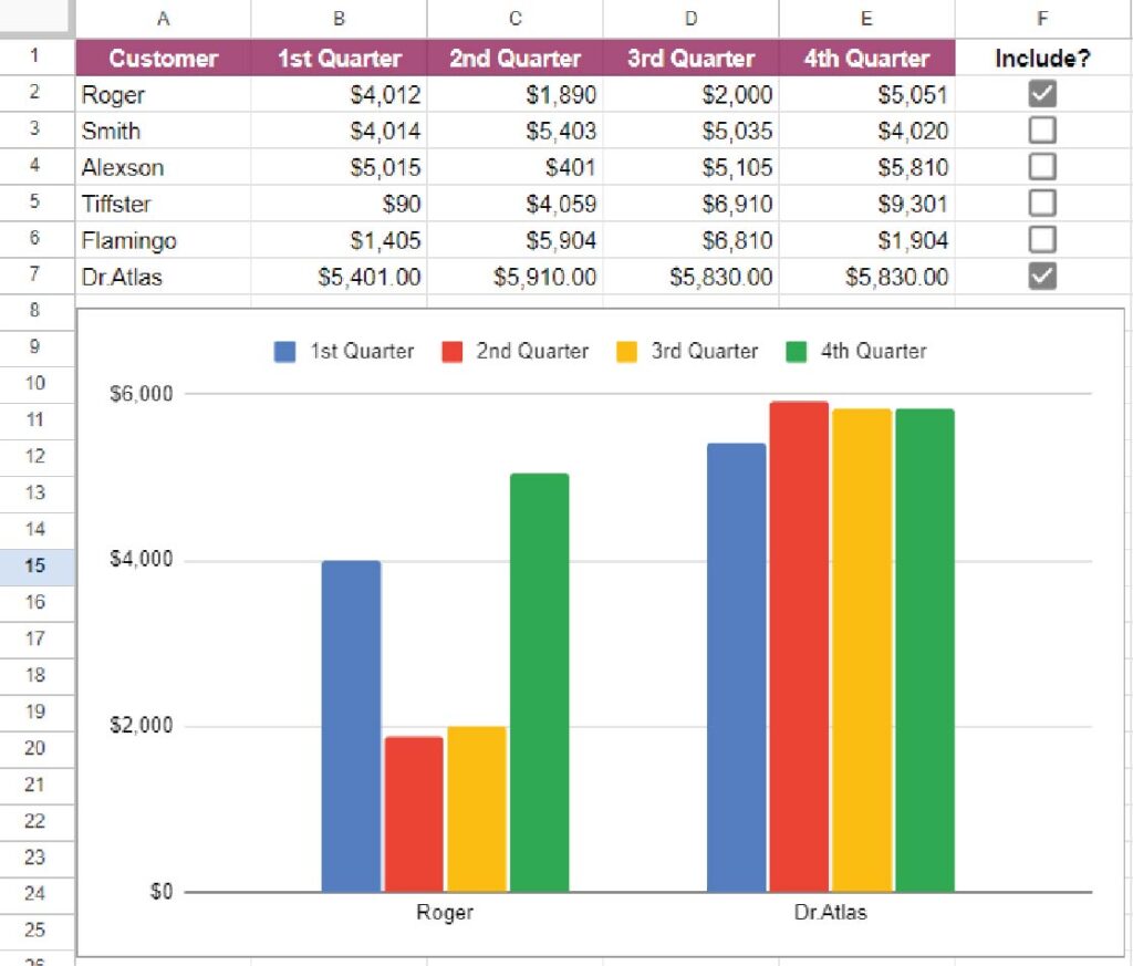
To make a dynamic chart, it’s much easier than it looks. We just need a duplicate table that only gathers the rows that are true, so this formula will work.
=QUERY(A1:F7,”where F = TRUE”,1)
Then highlight your duplicated table and make a chart.